How to Draw a X Y Z Plane

Most common coordinate organisation (geometry)

Analogy of a Cartesian coordinate plane. Iv points are marked and labeled with their coordinates: (2, iii) in greenish, (−3, 1) in crimson, (−1.5, −2.5) in blue, and the origin (0, 0) in purple.

A Cartesian coordinate arrangement (, ) in a aeroplane is a coordinate arrangement that specifies each betoken uniquely by a pair of numerical coordinates, which are the signed distances to the point from 2 fixed perpendicular oriented lines, measured in the same unit of length. Each reference coordinate line is called a coordinate axis or just axis (plural axes ) of the organisation, and the signal where they see is its origin, at ordered pair (0, 0). The coordinates tin can too be defined as the positions of the perpendicular projections of the point onto the 2 axes, expressed as signed distances from the origin.

One can use the aforementioned principle to specify the position of any point in three-dimensional space past three Cartesian coordinates, its signed distances to three mutually perpendicular planes (or, equivalently, by its perpendicular project onto three mutually perpendicular lines). In general, n Cartesian coordinates (an element of real north-infinite) specify the point in an n-dimensional Euclidean space for any dimension n. These coordinates are equal, up to sign, to distances from the point to n mutually perpendicular hyperplanes.

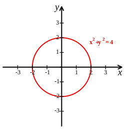
Cartesian coordinate system with a circle of radius 2 centered at the origin marked in red. The equation of a circle is (x − a)² + (y − b)ⁱⁱ = r ² where a and b are the coordinates of the centre (a, b) and r is the radius.

The invention of Cartesian coordinates in the 17th century by René Descartes (Latinized name: Cartesius) revolutionized mathematics by providing the first systematic link between Euclidean geometry and algebra. Using the Cartesian coordinate arrangement, geometric shapes (such as curves) can be described by Cartesian equations: algebraic equations involving the coordinates of the points lying on the shape. For example, a circumvolve of radius 2, centered at the origin of the plane, may be described every bit the ready of all points whose coordinates x and y satisfy the equation 10 ² + y ² = 4.

Cartesian coordinates are the foundation of analytic geometry, and provide enlightening geometric interpretations for many other branches of mathematics, such as linear algebra, complex analysis, differential geometry, multivariate calculus, group theory and more. A familiar instance is the concept of the graph of a part. Cartesian coordinates are also essential tools for most applied disciplines that deal with geometry, including astronomy, physics, technology and many more than. They are the most mutual coordinate organization used in calculator graphics, computer-aided geometric blueprint and other geometry-related data processing.

History [edit]

The adjective Cartesian refers to the French mathematician and philosopher René Descartes, who published this idea in 1637. It was independently discovered past Pierre de Fermat, who also worked in three dimensions, although Fermat did not publish the discovery.^[ane] The French cleric Nicole Oresme used constructions similar to Cartesian coordinates well before the time of Descartes and Fermat.^[2]

Both Descartes and Fermat used a single axis in their treatments and take a variable length measured in reference to this axis. The concept of using a pair of axes was introduced later, after Descartes' La Géométrie was translated into Latin in 1649 past Frans van Schooten and his students. These commentators introduced several concepts while trying to clarify the ideas contained in Descartes' piece of work.^[iii]

The development of the Cartesian coordinate arrangement would play a primal role in the evolution of the calculus by Isaac Newton and Gottfried Wilhelm Leibniz.^[4] The two-coordinate clarification of the plane was later on generalized into the concept of vector spaces.^[five]

Many other coordinate systems take been developed since Descartes, such every bit the polar coordinates for the plane, and the spherical and cylindrical coordinates for iii-dimensional space.

Description [edit]

One dimension [edit]

Choosing a Cartesian coordinate system for a one-dimensional space—that is, for a directly line—involves choosing a point O of the line (the origin), a unit of length, and an orientation for the line. An orientation chooses which of the two half-lines determined past O is the positive and which is negative; nosotros and so say that the line "is oriented" (or "points") from the negative half towards the positive half. Then each point P of the line can be specified by its distance from O, taken with a + or − sign depending on which half-line contains P.

A line with a chosen Cartesian arrangement is called a number line. Every real number has a unique location on the line. Conversely, every point on the line tin be interpreted as a number in an ordered continuum such every bit the real numbers.

Two dimensions [edit]

A Cartesian coordinate system in two dimensions (likewise chosen a rectangular coordinate system or an orthogonal coordinate organisation ^[6]) is divers by an ordered pair of perpendicular lines (axes), a single unit of length for both axes, and an orientation for each axis. The point where the axes meet is taken equally the origin for both, thus turning each axis into a number line. For whatsoever indicate P, a line is drawn through P perpendicular to each centrality, and the position where it meets the axis is interpreted as a number. The two numbers, in that called order, are the Cartesian coordinates of P. The contrary structure allows one to determine the point P given its coordinates.

The first and second coordinates are called the abscissa and the ordinate of P, respectively; and the indicate where the axes run into is called the origin of the coordinate organisation. The coordinates are normally written as two numbers in parentheses, in that order, separated past a comma, equally in (3, −x.five). Thus the origin has coordinates (0, 0), and the points on the positive half-axes, one unit abroad from the origin, have coordinates (1, 0) and (0, ane).

In mathematics, physics, and engineering science, the commencement axis is commonly defined or depicted as horizontal and oriented to the right, and the second axis is vertical and oriented up. (Even so, in some computer graphics contexts, the ordinate axis may be oriented downwards.) The origin is often labeled O, and the two coordinates are often denoted by the messages 10 and Y, or x and y. The axes may so be referred to as the 10-axis and Y-axis. The choices of messages come from the original convention, which is to use the latter role of the alphabet to indicate unknown values. The beginning part of the alphabet was used to designate known values.

A Euclidean aeroplane with a chosen Cartesian coordinate system is called a Cartesian plane . In a Cartesian airplane i can define canonical representatives of certain geometric figures, such as the unit circle (with radius equal to the length unit, and middle at the origin), the unit of measurement square (whose diagonal has endpoints at (0, 0) and (1, i)), the unit hyperbola, and so on.

The two axes divide the plane into 4 right angles, called quadrants. The quadrants may be named or numbered in various ways, but the quadrant where all coordinates are positive is usually called the showtime quadrant.

If the coordinates of a point are (x, y), then its distances from the 10-centrality and from the Y-axis are |y| and |x|, respectively; where |...| denotes the accented value of a number.

Three dimensions [edit]

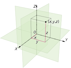
A three dimensional Cartesian coordinate system, with origin O and axis lines 10, Y and Z, oriented every bit shown past the arrows. The tick marks on the axes are 1 length unit autonomously. The blackness dot shows the point with coordinates $x = 2$ , $y = 3$ , and $z = 4$ , or $(2, 3, 4)$ .

A Cartesian coordinate system for a three-dimensional space consists of an ordered triplet of lines (the axes) that become through a mutual betoken (the origin), and are pair-wise perpendicular; an orientation for each axis; and a single unit of measurement of length for all iii axes. As in the 2-dimensional instance, each axis becomes a number line. For any point P of space, i considers a hyperplane through P perpendicular to each coordinate centrality, and interprets the point where that hyperplane cuts the axis as a number. The Cartesian coordinates of P are those three numbers, in the chosen club. The reverse construction determines the point P given its three coordinates.

Alternatively, each coordinate of a bespeak P can be taken every bit the distance from P to the hyperplane divers by the other two axes, with the sign determined past the orientation of the corresponding centrality.

Each pair of axes defines a coordinate hyperplane. These hyperplanes divide space into 8 trihedra, called octants.

The octants are: $\scriptstyle |(+x,+y,+z)|(-x,+y,+z)|(+x,+y,-z)|(-x,+y,-z)|(+x,-y,+z)|(-x,-y,+z)|(+ten,-y,-z)|(-ten,-y,-z)|$

The coordinates are usually written as three numbers (or algebraic formulas) surrounded by parentheses and separated by commas, as in $(iii, -2.five, 1)$ or $(t, u + v, π /ii)$ . Thus, the origin has coordinates $(0, 0, 0)$ , and the unit points on the iii axes are $(1, 0, 0)$ , $(0, one, 0)$ , and $(0, 0, 1)$ .

There are no standard names for the coordinates in the three axes (yet, the terms abscissa, ordinate and applicate are sometimes used). The coordinates are often denoted by the messages X, Y, and Z, or 10, y, and z. The axes may then be referred to as the X-axis, Y-axis, and Z-centrality, respectively. And so the coordinate hyperplanes can be referred to as the XY-plane, YZ-plane, and XZ-aeroplane.

In mathematics, physics, and engineering contexts, the showtime two axes are often defined or depicted equally horizontal, with the tertiary axis pointing upwards. In that case the third coordinate may be called height or altitude. The orientation is usually called and so that the 90 degree bending from the offset centrality to the second axis looks counter-clockwise when seen from the signal $(0, 0, 1)$ ; a convention that is commonly chosen the right mitt rule.

The coordinate surfaces of the Cartesian coordinates $(x, y, z)$ . The z-axis is vertical and the x-centrality is highlighted in green. Thus, the crimson hyperplane shows the points with $10 = 1$ , the blue hyperplane shows the points with $z = 1$ , and the xanthous hyperplane shows the points with $y = -i$ . The three surfaces intersect at the bespeak P (shown as a black sphere) with the Cartesian coordinates $(ane, -one, ane$ ).

Higher dimensions [edit]

Since Cartesian coordinates are unique and non-ambiguous, the points of a Cartesian plane can be identified with pairs of real numbers; that is, with the Cartesian product $\mathbb {R} ^{2}=\mathbb {R} \times \mathbb {R}$ , where $\mathbb {R}$ is the prepare of all real numbers. In the same way, the points in whatsoever Euclidean space of dimension n be identified with the tuples (lists) of n real numbers; that is, with the Cartesian production $\mathbb {R} ^{n}$ .

Generalizations [edit]

The concept of Cartesian coordinates generalizes to allow axes that are non perpendicular to each other, and/or different units along each axis. In that example, each coordinate is obtained past projecting the point onto one axis along a direction that is parallel to the other axis (or, in full general, to the hyperplane defined past all the other axes). In such an oblique coordinate system the computations of distances and angles must be modified from that in standard Cartesian systems, and many standard formulas (such as the Pythagorean formula for the distance) do not concord (see affine airplane).

Notations and conventions [edit]

The Cartesian coordinates of a point are unremarkably written in parentheses and separated by commas, as in (ten, v) or (3, 5, 7). The origin is often labelled with the upper-case letter letter O. In analytic geometry, unknown or generic coordinates are often denoted by the letters (x, y) in the plane, and (x, y, z) in three-dimensional space. This custom comes from a convention of algebra, which uses letters near the end of the alphabet for unknown values (such as the coordinates of points in many geometric problems), and messages near the beginning for given quantities.

These conventional names are often used in other domains, such equally physics and applied science, although other letters may be used. For case, in a graph showing how a pressure level varies with fourth dimension, the graph coordinates may exist denoted p and t. Each centrality is ordinarily named after the coordinate which is measured forth it; and then i says the x-axis, the y-axis, the t-centrality, etc.

Another common convention for coordinate naming is to employ subscripts, as (x _ane, x ₂, ..., 10 _n) for the n coordinates in an due north-dimensional space, especially when n is greater than three or unspecified. Some authors adopt the numbering (x ₀, 10 ₁, ..., x _n−ane). These notations are especially advantageous in computer programming: by storing the coordinates of a indicate as an array, instead of a tape, the subscript can serve to index the coordinates.

In mathematical illustrations of two-dimensional Cartesian systems, the kickoff coordinate (traditionally chosen the abscissa) is measured along a horizontal axis, oriented from left to right. The second coordinate (the ordinate) is and so measured along a vertical axis, unremarkably oriented from lesser to top. Young children learning the Cartesian system, commonly learn the social club to read the values before cementing the x-, y-, and z-axis concepts, by starting with 2D mnemonics (for example, 'Walk forth the hall then up the stairs' akin to directly across the x-axis then up vertically along the y-axis).^[7]

Calculator graphics and image processing, still, often utilise a coordinate organization with the y-axis oriented downwards on the computer display. This convention adult in the 1960s (or earlier) from the fashion that images were originally stored in display buffers.

For three-dimensional systems, a convention is to portray the xy-aeroplane horizontally, with the z-axis added to stand for height (positive up). Furthermore, in that location is a convention to orient the x-axis toward the viewer, biased either to the right or left. If a diagram (3D projection or 2d perspective drawing) shows the x- and y-axis horizontally and vertically, respectively, then the z-axis should be shown pointing "out of the page" towards the viewer or camera. In such a 2D diagram of a 3D coordinate system, the z-centrality would appear every bit a line or ray pointing down and to the left or downwardly and to the correct, depending on the presumed viewer or camera perspective. In any diagram or display, the orientation of the 3 axes, equally a whole, is arbitrary. However, the orientation of the axes relative to each other should ever comply with the correct-hand rule, unless specifically stated otherwise. All laws of physics and math assume this correct-handedness, which ensures consistency.

For 3D diagrams, the names "abscissa" and "ordinate" are rarely used for x and y, respectively. When they are, the z-coordinate is sometimes chosen the applicate. The words abscissa, ordinate and applicate are sometimes used to refer to coordinate axes rather than the coordinate values.^[vi]

Quadrants and octants [edit]

The iv quadrants of a Cartesian coordinate system

The axes of a 2-dimensional Cartesian organization divide the airplane into four infinite regions, called quadrants,^{[half dozen]} each bounded by two half-axes. These are often numbered from 1st to 4th and denoted by Roman numerals: I (where the coordinates both have positive signs), Ii (where the abscissa is negative − and the ordinate is positive +), III (where both the abscissa and the ordinate are −), and 4 (abscissa +, ordinate −). When the axes are drawn according to the mathematical custom, the numbering goes counter-clockwise starting from the upper correct ("north-e") quadrant.

Similarly, a three-dimensional Cartesian organization defines a division of infinite into eight regions or octants,^[six] according to the signs of the coordinates of the points. The convention used for naming a specific octant is to list its signs; for example, (+ + +) or (− + −). The generalization of the quadrant and octant to an arbitrary number of dimensions is the orthant, and a similar naming organization applies.

Cartesian formulae for the plane [edit]

Distance betwixt two points [edit]

The Euclidean distance between 2 points of the plane with Cartesian coordinates $(x_{i},y_{i})$ and $(x_{2},y_{2})$ is

d={\sqrt {(x_{2}-x_{1})^{2}+(y_{2}-y_{1})^{ii}}}.

This is the Cartesian version of Pythagoras's theorem. In three-dimensional space, the distance between points $(x_{1},y_{ane},z_{one})$ and $(x_{2},y_{2},z_{2})$ is

d={\sqrt {(x_{2}-x_{1})^{2}+(y_{ii}-y_{ane})^{ii}+(z_{2}-z_{1})^{two}}},

which can be obtained by two consecutive applications of Pythagoras' theorem.^[8]

Euclidean transformations [edit]

The Euclidean transformations or Euclidean motions are the (bijective) mappings of points of the Euclidean plane to themselves which preserve distances between points. There are iv types of these mappings (too called isometries): translations, rotations, reflections and glide reflections.^[nine]

Translation [edit]

Translating a set of points of the airplane, preserving the distances and directions between them, is equivalent to adding a stock-still pair of numbers (a, b) to the Cartesian coordinates of every bespeak in the set. That is, if the original coordinates of a point are (10, y), after the translation they will be

(10',y')=(x+a,y+b).

Rotation [edit]

To rotate a effigy counterclockwise around the origin by some angle $\theta$ is equivalent to replacing every point with coordinates (x,y) past the bespeak with coordinates (x',y'), where

x'=x\cos \theta -y\sin \theta

y'=x\sin \theta +y\cos \theta .

Thus:

(10',y')=((x\cos \theta -y\sin \theta \,),(x\sin \theta +y\cos \theta \,)).

Reflection [edit]

If (x, y) are the Cartesian coordinates of a betoken, and then (−x, y) are the coordinates of its reflection across the 2d coordinate axis (the y-axis), as if that line were a mirror. Likewise, (x, −y) are the coordinates of its reflection across the first coordinate axis (the ten-axis). In more generality, reflection beyond a line through the origin making an angle $\theta$ with the x-axis, is equivalent to replacing every point with coordinates (ten, y) by the betoken with coordinates (x′,y′), where

ten'=x\cos two\theta +y\sin 2\theta

y'=x\sin 2\theta -y\cos 2\theta .

Thus:

(x',y')=((x\cos ii\theta +y\sin 2\theta \,),(x\sin two\theta -y\cos 2\theta \,)).

Glide reflection [edit]

A glide reflection is the limerick of a reflection beyond a line followed by a translation in the direction of that line. It tin can be seen that the society of these operations does non affair (the translation tin can come kickoff, followed by the reflection).

General matrix form of the transformations [edit]

All affine transformations of the aeroplane tin can be described in a uniform manner by using matrices. For this purpose the coordinates $(x,y)$ of a indicate are commonly represented as the column matrix ${\begin{pmatrix}x\\y\finish{pmatrix}}.$ The event $(10',y')$ of applying an affine transformation to a point $(x,y)$ is given by the formula

{\brainstorm{pmatrix}ten'\\y'\end{pmatrix}}=A{\begin{pmatrix}x\\y\terminate{pmatrix}}+b,

where

A={\begin{pmatrix}A_{ane,1}&A_{ane,2}\\A_{2,1}&A_{2,2}\stop{pmatrix}}

is a 2×ii matrix and $b={\begin{pmatrix}b_{ane}\\b_{2}\cease{pmatrix}}$ is a column matrix.^[10] That is,

x'=xA_{1,1}+yA_{ane,1}+b_{i}

y'=xA_{ii,1}+yA_{2,2}+b_{ii}.

Amidst the affine transformations, the Euclidean transformations are characterized by the fact that the matrix $A$ is orthogonal; that is, its columns are orthogonal vectors of Euclidean norm one, or, explicitly,

A_{1,ane}A_{1,2}+A_{2,1}A_{2,2}=0

and

A_{1,ane}^{2}+A_{2,1}^{ii}=A_{i,2}^{2}+A_{2,2}^{2}=one.

This is equivalent to saying that $A$ times its transpose is the identity matrix. If these conditions exercise not hold, the formula describes a more general affine transformation.

The transformation is a translation if and only if $A$ is the identity matrix. The transformation is a rotation around some betoken if and only if $A$ is a rotation matrix, meaning that it is orthogonal and

A_{1,1}A_{2,2}-A_{2,1}A_{1,2}=1.

A reflection or glide reflection is obtained when,

A_{one,1}A_{2,two}-A_{2,1}A_{ane,ii}=-1.

Assuming that translations are not used (that is, $b_{ane}=b_{2}=0$ ) transformations tin can be equanimous by only multiplying the associated transformation matrices. In the general case, it is useful to employ the augmented matrix of the transformation; that is, to rewrite the transformation formula

{\begin{pmatrix}ten'\\y'\\1\end{pmatrix}}=A'{\begin{pmatrix}x\\y\\ane\end{pmatrix}},

where

A'={\begin{pmatrix}A_{ane,1}&A_{ane,ii}&b_{i}\\A_{two,1}&A_{2,2}&b_{2}\\0&0&1\end{pmatrix}}.

With this play a joke on, the composition of affine transformations is obtained by multiplying the augmented matrices.

Affine transformation [edit]

Effect of applying various 2D affine transformation matrices on a unit square (reflections are special cases of scaling)

Affine transformations of the Euclidean airplane are transformations that map lines to lines, only may alter distances and angles. As said in the preceding department, they tin can be represented with augmented matrices:

{\brainstorm{pmatrix}A_{i,one}&A_{2,1}&b_{1}\\A_{1,2}&A_{2,2}&b_{ii}\\0&0&1\end{pmatrix}}{\begin{pmatrix}x\\y\\one\terminate{pmatrix}}={\begin{pmatrix}x'\\y'\\1\end{pmatrix}}.

The Euclidean transformations are the affine transformations such that the 2×2 matrix of the $A_{i,j}$ is orthogonal.

The augmented matrix that represents the composition of 2 affine transformations is obtained by multiplying their augmented matrices.

Some affine transformations that are not Euclidean transformations have received specific names.

Scaling [edit]

An case of an affine transformation which is not Euclidean is given past scaling. To make a figure larger or smaller is equivalent to multiplying the Cartesian coordinates of every betoken by the same positive number m. If (x, y) are the coordinates of a bespeak on the original effigy, the corresponding point on the scaled figure has coordinates

(x',y')=(mx,my).

If m is greater than i, the figure becomes larger; if m is betwixt 0 and 1, it becomes smaller.

Shearing [edit]

A shearing transformation will button the pinnacle of a square sideways to class a parallelogram. Horizontal shearing is defined past:

(ten',y')=(x+ys,y)

Shearing tin can likewise be applied vertically:

(x',y')=(x,xs+y)

Orientation and handedness [edit]

In two dimensions [edit]

Fixing or choosing the x-axis determines the y-axis up to direction. Namely, the y-axis is necessarily the perpendicular to the x-axis through the point marked 0 on the 10-axis. Simply there is a choice of which of the two half lines on the perpendicular to designate as positive and which equally negative. Each of these two choices determines a different orientation (also called handedness) of the Cartesian plane.

The usual mode of orienting the plane, with the positive ten-axis pointing right and the positive y-axis pointing upwards (and the x-axis being the "kickoff" and the y-axis the "2nd" axis), is considered the positive or standard orientation, also called the right-handed orientation.

A commonly used mnemonic for defining the positive orientation is the right-hand rule. Placing a somewhat closed right mitt on the plane with the thumb pointing upwardly, the fingers signal from the x-axis to the y-axis, in a positively oriented coordinate organization.

The other way of orienting the plane is following the left paw rule, placing the left hand on the aeroplane with the thumb pointing upwardly.

When pointing the thumb away from the origin along an axis towards positive, the curvature of the fingers indicates a positive rotation forth that axis.

Regardless of the rule used to orient the aeroplane, rotating the coordinate organization will preserve the orientation. Switching whatever i axis will contrary the orientation, just switching both will get out the orientation unchanged.

In iii dimensions [edit]

Fig. 7 – The left-handed orientation is shown on the left, and the right-handed on the right.

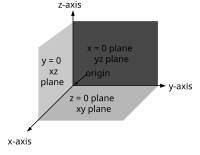
Fig. 8 – The correct-handed Cartesian coordinate system indicating the coordinate planes.

Once the x- and y-axes are specified, they determine the line forth which the z-axis should lie, but there are 2 possible orientation for this line. The two possible coordinate systems which issue are called 'right-handed' and 'left-handed'. The standard orientation, where the xy-plane is horizontal and the z-axis points upwardly (and the x- and the y-centrality form a positively oriented ii-dimensional coordinate system in the xy-plane if observed from above the xy-plane) is called right-handed or positive.

3D Cartesian coordinate handedness

The name derives from the right-hand rule. If the index finger of the correct hand is pointed forrard, the center finger bent inward at a right angle to it, and the thumb placed at a right angle to both, the three fingers betoken the relative orientation of the x-, y-, and z-axes in a right-handed system. The thumb indicates the 10-axis, the index finger the y-centrality and the center finger the z-centrality. Conversely, if the same is done with the left manus, a left-handed organisation results.

Figure 7 depicts a left and a right-handed coordinate arrangement. Because a 3-dimensional object is represented on the ii-dimensional screen, baloney and ambiguity result. The axis pointing downward (and to the right) is also meant to betoken towards the observer, whereas the "heart"-centrality is meant to signal away from the observer. The red circle is parallel to the horizontal xy-aeroplane and indicates rotation from the x-axis to the y-centrality (in both cases). Hence the reddish arrow passes in front of the z-axis.

Figure 8 is another attempt at depicting a right-handed coordinate system. Once again, there is an ambiguity caused by projecting the three-dimensional coordinate system into the plane. Many observers see Figure 8 equally "flipping in and out" between a convex cube and a concave "corner". This corresponds to the two possible orientations of the space. Seeing the effigy every bit convex gives a left-handed coordinate arrangement. Thus the "correct" way to view Figure 8 is to imagine the x-axis as pointing towards the observer and thus seeing a concave corner.

Representing a vector in the standard basis [edit]

A point in infinite in a Cartesian coordinate system may also exist represented by a position vector, which tin can be idea of as an arrow pointing from the origin of the coordinate system to the point.^[11] If the coordinates represent spatial positions (displacements), information technology is common to represent the vector from the origin to the indicate of interest as $\mathbf {r}$ . In 2 dimensions, the vector from the origin to the point with Cartesian coordinates (10, y) can be written every bit:

\mathbf {r} =x\mathbf {i} +y\mathbf {j} ,

where $\mathbf {i} ={\begin{pmatrix}1\\0\end{pmatrix}}$ and $\mathbf {j} ={\begin{pmatrix}0\\i\end{pmatrix}}$ are unit vectors in the management of the x-axis and y-axis respectively, generally referred to as the standard basis (in some application areas these may besides exist referred to as versors). Similarly, in three dimensions, the vector from the origin to the indicate with Cartesian coordinates $(ten,y,z)$ tin exist written as:^[12]

\mathbf {r} =x\mathbf {i} +y\mathbf {j} +z\mathbf {k} ,

where $\mathbf {i} ={\begin{pmatrix}i\\0\\0\end{pmatrix}},$ $\mathbf {j} ={\begin{pmatrix}0\\ane\\0\end{pmatrix}},$ and $\mathbf {k} ={\begin{pmatrix}0\\0\\one\end{pmatrix}}.$

At that place is no natural interpretation of multiplying vectors to obtain some other vector that works in all dimensions, however in that location is a way to utilize complex numbers to provide such a multiplication. In a 2-dimensional cartesian plane, identify the point with coordinates (x, y) with the complex number z = x + iy . Here, i is the imaginary unit of measurement and is identified with the bespeak with coordinates (0, ane), and so it is not the unit vector in the direction of the 10-axis. Since the complex numbers can exist multiplied giving another complex number, this identification provides a ways to "multiply" vectors. In a three-dimensional cartesian space a similar identification can be made with a subset of the quaternions.

Applications [edit]

Cartesian coordinates are an abstraction that accept a multitude of possible applications in the real world. However, 3 constructive steps are involved in superimposing coordinates on a problem application.

Units of altitude must be decided defining the spatial size represented by the numbers used as coordinates.
An origin must be assigned to a specific spatial location or landmark, and
the orientation of the axes must be defined using available directional cues for all only one axis.

Consider as an example superimposing 3D Cartesian coordinates over all points on the Globe (that is, geospatial 3D). Kilometers are a proficient choice of units, since the original definition of the kilometer was geospatial, with 10,000 km equaling the surface distance from the equator to the Due north Pole. Based on symmetry, the gravitational centre of the Earth suggests a natural placement of the origin (which can be sensed via satellite orbits). The axis of Globe'south rotation provides a natural orientation for the Ten, Y, and Z axes, strongly associated with "up vs. down", so positive Z can adopt the direction from the geocenter to the Due north Pole. A location on the equator is needed to define the Ten-axis, and the prime number tiptop stands out as a reference orientation, so the X-centrality takes the orientation from the geocenter out to 0 degrees longitude, 0 degrees latitude. Note that with three dimensions, and 2 perpendicular axes orientations pinned down for X and Z, the Y-axis is determined past the first ii choices. In order to obey the right-hand dominion, the Y-axis must point out from the geocenter to ninety degrees longitude, 0 degrees latitude. From a longitude of −73.985656 degrees, a latitude 40.748433 degrees, and Earth radius of xl,000/2π km, and transforming from spherical to Cartesian coordinates, one can guess the geocentric coordinates of the Empire Country Building, $(x, y, z) = (ane,330.53 km, 4,635.75 km, 4,155.46 km)$ . GPS navigation relies on such geocentric coordinates.

In engineering projects, understanding on the definition of coordinates is a crucial foundation. I cannot assume that coordinates come predefined for a novel application, so knowledge of how to cock a coordinate system where there previously was no such coordinate arrangement is essential to applying René Descartes' thinking.

While spatial applications utilize identical units along all axes, in business organization and scientific applications, each axis may accept unlike units of measurement associated with it (such as kilograms, seconds, pounds, etc.). Although four- and higher-dimensional spaces are difficult to visualize, the algebra of Cartesian coordinates can be extended relatively hands to four or more than variables, so that certain calculations involving many variables can be washed. (This sort of algebraic extension is what is used to define the geometry of higher-dimensional spaces.) Conversely, it is often helpful to use the geometry of Cartesian coordinates in two or three dimensions to visualize algebraic relationships between two or three of many non-spatial variables.

The graph of a role or relation is the set of all points satisfying that function or relation. For a function of one variable, f, the set of all points $(x, y)$ , where $y = f (10)$ is the graph of the office f. For a function g of two variables, the fix of all points $(ten, y, z)$ , where $z = g (ten, y)$ is the graph of the function g. A sketch of the graph of such a function or relation would consist of all the salient parts of the function or relation which would include its relative extrema, its concavity and points of inflection, any points of discontinuity and its end behavior. All of these terms are more fully defined in calculus. Such graphs are useful in calculus to understand the nature and beliefs of a function or relation.

References [edit]

^ Bix, Robert A.; D'Souza, Harry J. "Analytic geometry". Encyclopædia Britannica . Retrieved 6 August 2017.
^ Kent, Alexander J.; Vujakovic, Peter (four October 2017). The Routledge Handbook of Mapping and Cartography. Routledge. ISBN9781317568216.
^ Burton 2011, p. 374
^ A Tour of the Calculus, David Berlinski
^ Axler, Sheldon (2015). Linear Algebra Done Correct - Springer. Undergraduate Texts in Mathematics. p. 1. doi:10.1007/978-3-319-11080-half dozen. ISBN978-3-319-11079-0.
^ ^a ^b ^c ^d "Cartesian orthogonal coordinate system". Encyclopedia of Mathematics . Retrieved 6 August 2017.
^ "Charts and Graphs: Choosing the Right Format". www.mindtools.com . Retrieved 29 August 2017.
^ Hughes-Hallett, Deborah; McCallum, William G.; Gleason, Andrew M. (2013). Calculus : Unmarried and Multivariable (6 ed.). John wiley. ISBN978-0470-88861-ii.
^ Smart 1998, Chap. 2
^ Brannan, Esplen & Gray 1998, pg. 49
^ Brannan, Esplen & Gray 1998, Appendix 2, pp. 377–382
^ David J. Griffiths (1999). Introduction to Electrodynamics . Prentice Hall. ISBN978-0-13-805326-0.

Sources [edit]

Brannan, David A.; Esplen, Matthew F.; Gray, Jeremy J. (1998), Geometry, Cambridge: Cambridge Academy Printing, ISBN978-0-521-59787-vi
Burton, David 1000. (2011), The History of Mathematics/An Introduction (7th ed.), New York: McGraw-Hill, ISBN978-0-07-338315-6
Smart, James R. (1998), Modern Geometries (5th ed.), Pacific Grove: Brooks/Cole, ISBN978-0-534-35188-v

External links [edit]

Cartesian Coordinate Organisation
MathWorld clarification of Cartesian coordinates
Coordinate Converter – converts between polar, Cartesian and spherical coordinates
Coordinates of a betoken Interactive tool to explore coordinates of a point
open source JavaScript class for second/3D Cartesian coordinate system manipulation

oharanstruch96.blogspot.com

Source: https://en.wikipedia.org/wiki/Cartesian_coordinate_system